6. Improvement and Extension of Programs

Continuing from the previous chapter, we will extend the kinematics simulation of particles. Specifically, we will add particles that bounce off the edge of the screen instead of disappearing.

It is easy to modify the particle.py code in the previous chapter to make such a change. It only takes a few lines of code, so it can be done in a few minutes by a skilled person.

However, in general, the larger and more complex the program, the more difficult it becomes to modify and extend. If you don’t think things through carefully, your program will grow into an unmanageable mess in no time.

In this chapter, we will look at some of the most common techniques for continuous program maintenance and extension, specifically class inheritance and object composition. We will also introduce unit testing to help you modify your programs.

If I am developing a disposable program that I am only going to use temporarily, I don’t have to think too seriously about it and I can just make it quickly, right?

If it’s really a disposable program, that’s fine, but it’s quite common to suddenly need to modify or add a new function to a program that was created with that intention. There is no harm in keeping this in mind to some extent.

6.1. Module

Since the program is getting larger and larger, we’ll split it into several files before we start modifying it or adding features.

Create a new file projectile_main.py and move the definition of the class AppMain to it. Leave World and Particle in particle.py.

particle.py (ver 12.0)

import pygame


class World:
    def __init__(self, width, height, dt, gy):
        self.width = width
        self.height = height
        self.dt = dt
        self.gy = gy


class Particle:
    def __init__(self, pos, vel, world, radius=10.0, color="green"):
        self.is_alive = True
        self.x, self.y = pos
        self.vx, self.vy = vel
        self.world = world
        self.radius = radius
        self.color = pygame.Color(color)

    def update(self):
        self.vy += self.world.gy * self.world.dt
        self.x += self.vx * self.world.dt
        self.y += self.vy * self.world.dt
        if self.x < 0 or self.x > self.world.width or self.y > self.world.height:
            self.is_alive = False

    def draw(self, screen):
        pygame.draw.circle(screen, self.color, (self.x, self.y), self.radius)

particle_main.py (ver 12.0)

import random
import pygame
import particle


class AppMain:
    def __init__(self):
        pygame.init()
        width, height = 600, 400
        self.screen = pygame.display.set_mode((width, height))
        self.world = particle.World(width, height, dt=1.0, gy=0.5)
        self.particle_list = []

    def update(self):
        for p in self.particle_list:
            p.update()
        self.particle_list[:] = [p for p in self.particle_list if p.is_alive]

    def draw(self):
        self.screen.fill(pygame.Color("black"))
        for p in self.particle_list:
            p.draw(self.screen)
        pygame.display.update()

    def add_particle(self, pos, button):
        if button == 1:
            vx = random.uniform(-10, 10)
            vy = random.uniform(-10, 0)
            p = particle.Particle(pos, (vx, vy), self.world)
            self.particle_list.append(p)

    def run(self):
        clock = pygame.time.Clock()

        while True:
            frames_per_second = 60
            clock.tick(frames_per_second)

            should_quit = False
            for event in pygame.event.get():
                if event.type == pygame.QUIT:
                    should_quit = True
                elif event.type == pygame.KEYDOWN:
                    if event.key == pygame.K_ESCAPE:
                        should_quit = True
                elif event.type == pygame.MOUSEBUTTONDOWN:
                    self.add_particle(event.pos, event.button)
            if should_quit:
                break

            self.update()
            self.draw()

        pygame.quit()


if __name__ == "__main__":
    app = AppMain()
    app.run()

Lines 2-3

We put import particle at the top of projectile_main.py to use the definitions in particle.py.

Also, since only AppMain uses random.uniform, import random here instead of in particle.py.

Line 11

World and Particle are now part of the particle module. So they should be rewritten as particle.World and particle.Particle, respectively. (Or you need to change the import line to from particle import World, Particle)

Now you have your own module particle, which is separated from the program projectile_main.py that uses it.

Run it and make sure it works as before, then stage both files in VSCode’s Source Control sidebar and commit them.

When I try Run ‣ Run Without Debugging, nothing is displayed and no error occurs.

Is particle_main.py displayed in the editor area of VSCode?

In our pre-configured development environment, when you execute Run ‣ Run Without Debugging, it runs the file that is active in the editor area; if particle.py is active, it will only define the classes and exit.

If you don’t want to activate it each time you want to run particle_main.py, you can add a configuration to always run this file as follows

• Execute Run ‣ Add Configuration, then select Add Configuration in the bottom right popup
• Specify particle_main.py in "program": "${file}".

The created Configuration can be selected at the top of the Run sidebar.

I wonder why the version number of particle_main.py is 12.0, although it is a new file.

Think of it as the version number of the entire folder.

When a program is divided into multiple source files, it is important to keep track of the versions of all the files synchronously. If you don’t, you will end up in the unfortunate situation like “Which version of particle.py can run this version?”

In fact, a commit of Git can contain multiple files, and they are managed together.

In this textbook, if there are two (or three or more) files with the same version number, they are the files at the same point in time.

6.2. Unit Testing

6.2.1. Psychological Effects of Tests

When adding functionality to an existing program, or modifying it without changing its functionality (refactoring), it is necessary to make sure that the original functionality is not broken. And in a large program, this is more difficult than it seems.

It’s not uncommon to create a new function and think “Okay, it works,” only to find out after a while that there is a bug in the existing function (and by that time, you don’t remember what you changed).

After you repeat such experiences, you will have a psychological tendency to think “I don’t want to change the code that is working well now.” Even if you know that the code could be rewritten in a better way, you will want to postpone the modification. As a result, when the need to change the function arises, it is not possible to fix the problem cleanly, and ad hoc revisions are repeated, resulting in a negative spiral that becomes increasingly unmanageable.

One way to prevent such a situation from happening is to write tests. Prepare a small set of programs to check whether a part of the program (e.g., a function or a method) returns the correct result, and run them frequently (or, if you want, automatically whenever a modification occurs). In this way, the psychological barrier is much lowered, as you can organize your program with confidence that the original functionality is not broken, at least as far as the tests cover.

In the pre-configured environment for this course, we have already installed a tool called pytest for testing Python programs. Let’s give it a try.

Create a new file test_particle.py and save it with the following code.

test_particle.py (ver 13.0)

import particle


def test_particle_move():
    width, height = 600, 400
    dt, g = 2, 4
    w = particle.World(width, height, dt, g)
    x0, y0, vx0, vy0 = 0, 0, 5, 10
    p = particle.Particle((x0, y0), (vx0, vy0), w)
    p.update()
    assert p.x == x0 + vx0 * dt
    assert p.y == y0 + (vy0 + g * dt) * dt
    p.update()
    assert p.x == x0 + 2 * vx0 * dt
    assert p.y == y0 + (vy0 + g * dt) * dt + (vy0 + 2 * g * dt) * dt

At the command prompt (or in a terminal in VSCode), execute:

C:\cs1\projects\particle>pytest

It automatically detects and executes functions whose names start with test in files whose names start with test.

The content of the function is almost as you can see. The important part is the assert statement that we have sometimes used in previous exercises. This statement checks whether the position of the Particle (attributes x and y) updated by one time step from the initial state is equal to the expected one, and whether it is also correct after one more time step update. If there is a discrepancy, an error occurs.

This kind of testing to check the behavior of a single function or method, or at most a class, is called unit testing. Unit testing is fundamentally different from integration testing, which tests the combination of multiple components, and larger-scale system-level testing, and is not intended for quality assurance or evaluation of programs. It is a tool to help developers in their day-to-day programming.

In the first place, there is no guarantee that a program is absolutely correct just because it passes the tests. If I may be so bold as to say so without fear of being misunderstood, what can be expected from unit tests is not a guarantee of correctness, but a psychological effect to break the feeling of not wanting to change the working code.

Therefore, it does not have to be perfect. You don’t have to (and can’t) try to cover every condition. You don’t have to try to test every part of the program (you can’t). Start where you can, and do as much as you can. It will still help you a lot.

6.2.2. Running Tests from VSCode

The pytest execution function is built into VSCode, but it is disabled by default. Open the Explorer sidebar from the activity bar, right-click on the test_particle.py file, and select Run All Tests. You will see a popup saying “No test framework configured” in the lower right corner, so click Enable and Configure a Test Framework. When asked to Select a test framework/tool, select pytest, and select “. Root directory” when asked to Select the directory.

You should see Testing (flask icon) at the bottom of the activity bar. Click it to open the Testing sidebar, and click Run All Tests to run it. If you haven’t found any tests, click Discover Tests first. If the circle in front of each test item turns green, you have succeeded.

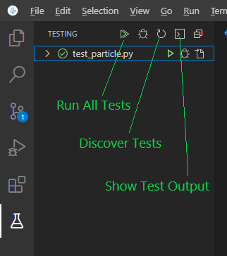
Unsuccessful tests will turn red. Try rewriting temporarily the test function or the update method of the Particle class to make them inconsisitent. Click “Show Test Output” in the sidebar to see the output in the panel area, and you can see which tests failed and how. (It is important to try to fail the test at least once after writing it, to reduce the risk of leaving a wrong test that does not work as a test in the first place)

When you see that a test fails, fix the program properly and make sure that the green signal lights up. When you are sure, add also test_particle.py in Git and commit.

6.2.3. Unrolling Multiple Test Parameters

Having only one initial condition tested is a bit worrisome. It is possible to prepare various initial values and run them through a for statement, but if you do so, it is difficult to know which condition failed when some of them failed. Also, it is a good rule not to make the test function too complicated, since having a bug in the test itself comes to nothing.

pytest has a function to run the same test function on multiple tuples of parameters.

test_particle.py (ver 14.0)

import pytest
import particle


@pytest.mark.parametrize("x0, y0, vx0, vy0", [
    (0, 0, 5, 10),
    (300, 200, -7, 12),
    (500, 300, -4, -10),
])
def test_particle_move(x0, y0, vx0, vy0):
    width, height = 600, 400
    dt, g = 2, 4
    w = particle.World(width, height, dt, g)

    p = particle.Particle((x0, y0), (vx0, vy0), w)
    p.update()
    assert p.x == x0 + vx0 * dt
    assert p.y == y0 + (vy0 + g * dt) * dt
    p.update()
    assert p.x == x0 + 2 * vx0 * dt
    assert p.y == y0 + (vy0 + g * dt) * dt + (vy0 + 2 * g * dt) * dt

In line 1, we import the pytest module, and the initial variables x0, y0, vx0, and vy0 defined in line 14 are moved to function arguments (line 10). The function is preceded by a mysterious incantation beginning with @ (lines 5-9).

In Python, you can define a decorator that can be placed just before a function definition to modify the behavior of the function. @ is a notation that calls the decorator.

Aside from the grammar, the pytest.mark.parametrize decorator allows you to give the arguments to the test function as a list of tuples. In this case, you can start with x0, y0, vx0, vy0 = 0, 0, 5, 0, then x0, y0, vx0, vy0 = 300, 200, -7, 12, and so on, and the test is run with these various initial values.

---

Let’s try some other tests. Since we know the analytical solution for a simple parabolic motion, it is natural to compare the results with the solution.

test_particle.py (ver 15.0)

@pytest.mark.parametrize("x0, y0, vx0, vy0", [
    (0, 0, 5, 10),
    (300, 200, -7, 12),
    (500, 300, -4, -10),
])
def test_particle_move_analytically(x0, y0, vx0, vy0):
    width, height = 600, 400
    dt, g = 1, 0.5
    w = particle.World(width, height, dt, g)

    p = particle.Particle((x0, y0), (vx0, vy0), w)
    N = 2000
    for _ in range(N):
        p.update()
    assert p.x == x0 + vx0 * (N * dt)
    py_discrete = y0 + vy0 * (N * dt) + 1/2 * g * N * (N + 1) * dt ** 2
    assert p.y == py_discrete
    py_continuous = y0 + vy0 * (N * dt) + 1/2 * g * N ** 2 * dt ** 2
    assert p.y == pytest.approx(py_continuous, 1e-3)

For the x-coordinate, there is no difficulty since the motion is constant velocity; for the y-coordinate, the example compares two solutions: py_discrete is the solution at \(t = N \Delta t\), where the solution is obtained by regarding the equation used in the update method of Particle as an recurrence formula. On the other hand, py_continous is the solution in continuous time. The latter is familiar to high school physics students.

\[\begin{split}y_\text{discrete} &= y(0) + \dot{y}(0) N \Delta t + \frac{1}{2} g N (N + 1) (\Delta t)^2\\ y_\text{continuous} &= y(0) + \dot{y}(0) N \Delta t + \frac{1}{2} g (N \Delta t)^2\end{split}\]

Of course, the latter does not exactly match to the actual result, but if N is large enough, we can expect them to be approximately equal. You can use the pytest.approx function, as in line 42, to make an approximate comparison. In this case, an error of up to \(10^{-3}\) times the absolute value of the correct answer is allowed.

Do I need to use pytest.approx only for approximate computation?

No, even an equation that should exactly hold true mathematically may not hold true due to numerical errors.

For example, the following equation should be mathematically valid, but the numerical results of the both sides do not agree:

>>> (0.1 + 0.5) + 0.2 == 0.1 + (0.5 + 0.2)
False

The above test_particle_move_analytically also fails if, for example, (0, 0, 5, 10.1) is specified as a parameter tuple.

Therefore, it is always safer to use pytest.approx unless you want to check the equivalence when numerical errors are involved.

Most of the test codes in this chapter work without pytest.approx, but it is better to understand that they just happen to work. Keep in mind that you may need pytest.approx if you want to try different parameters or change the calculation procedure.

What does _ in for _ in range(N): on line 36 mean?

It is a Python convention to declare that you define a variable but will not use it.

Here we just want to iterate N times. The numbers 0, 1, 2, … taken from range(N) will be assigned to the variable _, but the value will not be used in the loop.

If you use a named variable here, you may be worried when you read the code later wondering “Hey, I didn’t use this variable, is it really okay?” This is because an unused variable is a sign of a bug. In fact, VSCode in our pre-configured environment is set to warn about unused variables, so you should see an underline.

By using _ as the variable name, you can tell people reading the code later, or VSCode, that this variable is intentionally unused.

---

Finally, let’s test the is_alive attribute. In this case, it is easier and more reliable to give the expected results along with the initial conditions than to write a mathematical expression to determine if it should go off the screen or not. So we add an argument expected to have expected results.

test_particle.py (ver 16.0)

@pytest.mark.parametrize("x0, y0, vx0, vy0, expected", [
    (300, 200, 5, 10, True),
    (300, 200, -5, -10, True),
    (599, 200, 5, 10, False),
    (300, 399, 5, 10, False),
    (-1, 399, 5, 10, False),
    (0, 0, 5, 10, True),
    (0, 0, -5, 10, False),
])
def test_particle_liveness_after_move(x0, y0, vx0, vy0, expected):
    width, height = 600, 400
    dt, g = 1, 0.5
    w = particle.World(width, height, dt, g)
    p = particle.Particle((x0, y0), (vx0, vy0), w)
    p.update()
    assert p.is_alive == expected

Isn’t it really tedious?

It is really tedious.

In fact, if you want to write tests seriously, it often takes more time than writing the target code of the program.

So, I am not saying that you should always write tests when you write your own programs in this course. However, when we explain modern software development, we can’t leave testing out of the discussion. So please begin by just knowing that there are such concepts and techniques.

Then, for example, if you are worried about whether a function is written correctly, or if you want to modify a class but feel a psychological barrier, try unit testing, even if only partially.

In order to reduce the tediousness of writing tests, pytest has many features other than those described here. If you are interested in using them, please check them out.

I understand that unit tests are useful, but there are many things that we want to test but can’t seem to write tests for, such as a procedure depending on keyboard input, or one using random numbers.

There are a number of ways to get around this.

For example, later in this chapter, you will learn how to make a part of a program independent as an object, and replace it as needed. In the same way, you can write tests by putting the parts of the procedure you want to test, such as reading keyboard input or generating random numbers, into independent objects, and replacing them with ones that return known values only when testing. Such an object used for testing is called a mock object.

This concept can be used not only in unit testing but also in many other areas. For example, if you are writing a program that communicates with a certain piece of hardware, preparing a mock object that replaces the communication process will allow you to proceed with development even if you don’t have the actual hardware on hand.

Shouldn’t dt and g also be tested for different values?

It would be better to do so, but it would be too long, so it is omitted.

If you actually want to do this, you may want to use pytest.mark.parametrize in multiple layers. See test_particle.py (ver 24.0) for examples.

Clicking the Run All Tests icon every time is a pain.

There are also tools that automatically run tests whenever a file is modified.

Unfortunately, I can’t find any tools used within VSCode, but I’d like to introduce pytest-watch, which can be used from the command prompt.

It is easy to use. Open a new command prompt, navigate to the folder you are working on, and execute the ptw command there.

C:\cs1\projects>cd particle
C:\cs1\projects\particle>ptw

The test will automatically run and the displayed results will be updated every time it detects a change in the files. To stop it, type Ctrl + c.

6.3. Modification without Functional Changes

Now that we have written the unit tests, let’s modify the program. First, let’s look at an example of a modification that does not involve a functional change.

6.3.1. Refactoring into Methods

I’m sure you’re already familiar with refactoring into methods; We will refactor the processing at the screen boundary in Particle’s update method into a separate method. Of course, this is a prelude to adding a new feature (bouncing back) later.

Before you start modifying, make sure that your tests pass and that you have committed to Git.

particle.py (ver 17.0)

    def update(self):
        self.vy += self.world.gy * self.world.dt
        self.x += self.vx * self.world.dt
        self.y += self.vy * self.world.dt
        self.update_after_move()

    def update_after_move(self):
        if self.x < 0 or self.x > self.world.width or self.y > self.world.height:
            self.is_alive = False

The modification itself is easy. After it, make sure that the tests pass, run it with Run ‣ Run Without Debugging, and if everything is OK, commit the changes in Git.

It’s a simple task, but having tests makes you feel more secure. It’s also important to know that you can revert back to the original state if you need to, since you have committed the state just before modification.

Tweak the code a bit, run the tests, watch the signals go all green, and commit. If you can get your brain pumping with this repetition, you’re good to go.

6.3.2. Replacing with Objects of Higher Abstraction

Let’s make a few more substantive changes. pygame.math.Vector2 (Vector2) is a class that represents vectors in pygame. Try rewriting the code using this class.

particle.py (ver 18.0)

import pygame


class World:
    def __init__(self, width, height, dt, gy):
        self.width = width
        self.height = height
        self.dt = dt
        self.gravity_acc = pygame.math.Vector2(0, gy)


class Particle:
    def __init__(self, pos, vel, world, radius=10.0, color="green"):
        self.is_alive = True
        self.pos = pygame.math.Vector2(pos)
        self.vel = pygame.math.Vector2(vel)
        self.world = world
        self.radius = radius
        self.color = pygame.Color(color)

    def update(self):
        self.vel += self.world.gravity_acc * self.world.dt
        self.pos += self.vel * self.world.dt
        self.update_after_move()

The gravitational acceleration attribute in World and the position and velocity attributes in Particle are represented by Vector2, as the attributes gravity_acc, pos, and vel, respectively. Vector2 can be created by passing two arguments or a sequence of two elements (tuple, list, etc.).

Vector2 can represent element-wise addition and scalar multiplication with the operators + and *. This makes the kinematic calculations a bit simpler, as shown in lines 22-23. It will also make it easier to write various extensions in the future.

So try running the tests; you will see they fail. This is because the test functions use the Particle attributes x and y. In addition, the Particle’s method draw also uses the attributes x and y, so if you run particle_main.py, you will also get an error.

In other words, although we wanted to modify the program without changing the functionality, it has actually changed.

There are two options: we can either decide to discontinue the existing functionality (i.e., providing the position through attributes x and y), or we can modify it again such that this functionality is kept. We will take the latter option here. It is better to keep backward compatibility as much as possible.

One way is to keep x and y as attributes, and update them whenever pos is updated. This is still easy to do for the current program, but it is a lot of work for a program where pos is updated in multiple places. Also, if you modify the program in the future to update the pos in other places, you will be in trouble if you forget to do this.

This is why we use the @property decorator, which comes with Python. You may remember that a decorator is something you put in front of a function definition to change its behaviour. When applied to a method, @property replaces its name with a read-only attribute that is not a method, and the method is called when the attribute is read. It may be hard to understand. Let’s use a real-world example to illustrate.

particle.py (ver 18.0)

    def draw(self, screen):
        pygame.draw.circle(screen, self.color, (self.x, self.y), self.radius)

    @property
    def x(self):
        return self.pos.x

    @property
    def y(self):
        return self.pos.y

An object of type Vector2 allows reading and writing of its first and second elements through attributes x and y (or with [0] and [1] postfixed), respectively. If there were no @property in front of the line def x(self):, then method x would be defined such that the x-coordinate of object p of type Particle could be obtained through p.x(). However, this is still not backward compatible, since we have always written p.x. By putting @property, the method x() will be called automatically when the attribute x is read, and its return value will be obtained.

Now, make sure that the tests pass and particle_main.py can be executed before committing the changes. This completes the series of modifications.

Vector2 is a class defined in pygame, isn’t it? Why can we use the operators such as + and *?

Vector2 has __add__, __mul__, and other methods defined in it, which are called when the operators +, *, etc. are applied.

Methods with names between two underscores, such as __init__, are called special methods, and are called automatically under certain conditions. Similarly, for example, if vel and acc are Vector2-type objects and dt is a real number, the expression:

vel + acc * dt

is evaluated by calling:

vec.__add__(acc.__mul__(dt))

The mechanism for defining operator behavior in this way is generally called operator overloading. In C++, this is achieved by defining the methods operator+ and operator*. Some languages, such as Java, do not have operator overloading feature.

What if I want to replace an attribute with a method, as in this example, in a language that doesn’t have a feature like @property in Python?

There is no way to do that. In such a language, you should avoid reading and writing attribute variables directly from outside the class.

For example, C++ and Java are examples of such languages. In these languages, direct external access to object attribute variables such as p.x and p.y is not recommended in the first place. Even if it seems redundant, it is always better to access them through methods, such as p.x() and p.y(), so that you don’t have to worry about changing them to methods later on.

(See also the question from a passing Java programmer in Chapter 5)

I don’t understand the meaning of the word “property” used here. What’s the difference from “attribute”? They sound almost the same to me.

It’s better not to worry too much about it, because it’s a historical term.

The names for the equivalent of the attribute in Python vary from language to language: attribute, property, field, member variable, instance variable, … and so on.

Some languages among them started using the name “property” for the one which looks like just an attribute variable, but in fact is a method called behind the scenes, and other languages gradually adopted it.

6.4. Class Inheritance

6.4.1. Tentative Implementation of Bounce

Now, it’s time to change it so that it bounces on the left, right, and bottom boundaries of the screen. We can consider also the top boundary, but let’s assume that the sky is open as before (for no particular reason, but it’s fun to make it fly up and then come back down, isn’t it?)

The way to do this is to replace the processing of the method update_after_move that we refactored out earlier. Instead of setting is_alive to False when out of range, reverse the sign of vel.x or vel.y to make it a perfect elastic collision. If you want a imperfect elastic collision, just multiply by the restitution coefficient \(e\) as well.

We will define a class ConfinedParticle to represent such a particle. An easy way to do this would be to copy-paste the Particle code, rename it to ConfinedParticle, and make the necessary modifications. However, copying and pasting everything which is completely unchanged except the update_after_move method would be too wasteful. When you want to make common modifications to both classes later (for example, you want to modify the draw method to make it look better, or you find a bug in a common part), you will have to make the same modifications to both classes.

This is why we use a mechanism called class inheritance. Add the following code to particle.py.

particle.py (ver 19.0)

class ConfinedParticle(Particle):
    def update_after_move(self):
        e = 0.95
        if self.pos.x < 0 or self.pos.x > self.world.width:
            self.vel.x *= -e
        if self.pos.y > self.world.height:
            self.vel.y *= -e

This defines a ConfinedParticle. It is important to note that (Particle) is written after ConfinedParticle in line 42. This means that ConfinedParticle inherits all the definitions of Particle. It then overrides only the update_after_move method, which is redefined. In the new definition, the restitution coefficient is set to e, and vel.x is multiplied by -e when the particle hits the wall on either side, and vel.y is multiplied by -e when the particle hits the floor. The rest of the methods are exactly the same as those of Particle.

In this situation, ConfinedParticle is said to inherit from Particle. ConfinedParticle is called a sub class, a child class, or a derived class of Particle. Conversely, Particle is called the super class, parent class, or base class of ConfinedParticle.

If you rewrite the user code of the particle module, i.e., the part in particle_main.py that creates Particle type objects, so that ConfinedParticle is used instead of Particle, you should be able to see something working.

particle_main.py (ver 19.0)

    def add_particle(self, pos, button):
        if button == 1:
            vx = random.uniform(-10, 10)
            vy = random.uniform(-10, 0)
            p = particle.ConfinedParticle(pos, (vx, vy), self.world)
            self.particle_list.append(p)

6.4.2. Reconsidering the Bounce Processing

If you run the modified program for a while, you will notice that there are a few things that are not quite right. First of all, it doesn’t take the size of the particle into account, which makes it a bit strange. When the size is taken into account, the result looks like this.

particle.py (ver 20.0)

class ConfinedParticle(Particle):
    def update_after_move(self):
        e = 0.95
        if self.x < 0 + self.radius or self.x > self.world.width - self.radius:
            self.vel.x *= -e
        if self.y > self.world.height - self.radius:
            self.vel.y *= -e

In short, think of it as a wall that has moved inward by the radius. If we start considering the size of a particle, it may not be strictly a “particle”, but we don’t care.

Some of you may have noticed that there are still some discomfort. If you don’t, try a smaller restitution coefficient, e.g. e = 0.5. The following two problems become apparent.

• The velocity component, which should be multiplied by -e, may suddenly become zero.
• After repetition, it becomes slower and slower, settles on the floor, and then sinks into the floor.

To understand the cause of the first problem, put a breakpoint on the lines self.vel.x *= -e and self.vel.y *= -e (lines 46 and 48) and follow them in the debugger. You will see that these are executed multiple times in a single collision.

Since this simulation is run in discrete time, collisions generally occur when the object is slightly deeper into the wall. When a collision occurs, the velocity reverses, but there is a possibility that it will still be inside the wall at the next time step, in which case it will reverse and go into the wall again, and then it will flip again but it will still not get out of the wall, and so on.

Once the cause is known, the solution is simple: consider also the velocity as a collision condition. For example, if the wall is on the right side, the attribute vel.x must be positive for collision to occur.

The second problem is a bit confusing, but it stems from the fact that there is no fundamental mechanism for balancing the forces when the object is stationary on the floor. There is always a gravitational force on a particle, and the floor must provide a normal force to balance it, but there is no such force in this simulator.

As a countermeasure, we can avoid this problem by forcing the object to move its position to the floor only when a collision occurs in the y direction.

These two measures can be incorporated as follows.

particle.py (ver 21.0)

class ConfinedParticle(Particle):
    def update_after_move(self):
        e = 0.95
        if (self.x < 0 + self.radius and self.vel.x < 0) or \
           (self.x > self.world.width - self.radius and self.vel.x > 0):
            self.vel.x *= -e
        if self.y > self.world.height - self.radius and self.vel.y > 0:
            self.vel.y *= -e
            # constrain particle on or above the floor
            self.pos.y = self.world.height - self.radius

Note that in lines 45-46, the condition is too long and wrapped with \.

Not only is it long, but there are too many dot operators in it, making it difficult to read. In this case, you can use a local variable with a concise name.

particle.py (ver 22.0)

class ConfinedParticle(Particle):
    def update_after_move(self):
        x, y = self.x, self.y
        vx, vy = self.vel.x, self.vel.y
        width, height = self.world.width, self.world.height
        radius = self.radius
        e = 0.95
        if (x < 0 + radius and vx < 0) or (x > width - radius and vx > 0):
            self.vel.x *= -e
        if y > height - radius and vy > 0:
            self.vel.y *= -e
            # constrain particle on or above the floor
            self.pos.y = height - radius

Can’t I replace also the left hand side of the assignment with a local variable with a concise name?

No, you can’t. It will not work.

Try to imagine what happens if you write, for example, vx *= -e for self.vel.x *= -e recalling the “baggage tag” model.

The “tag” vx does not point to self.vel.x, but to the integer data that self.vel.x points to. vx *= -e causes vx to point to the new integer data, but self.vel.x still points to the original integer data.

Rewriting with local variables is a kind of refactoring, right? Don’t we have to write tests?

Because it will get long, I skipped it. But if you’re interested, read the rest of this answer (test_particle.py ver 21.0).

We create three test functions, one for bouncing off the wall, one for bouncing off the floor, and one for not being bounced off, as follows. We have found that it is important to make sure that the object does not bounce again immediately after it bounces, so we test movements for two time steps.

The recommended procedure is to verify that the test passes with particle.py ver 21.0, and then modify it into ver 22.0 while checking the test keeps passing.

test_particle.py (ver 21.0)

@pytest.mark.parametrize("x0, y0, vx0, vy0", [
    (600, 200, 5, 0),
    (0, 200, -7, 0),
])
def test_confined_particle_on_wall(x0, y0, vx0, vy0):
    dt, g = 1, 0.5
    w = particle.World(600, 400, dt, g)
    e = 0.95
    p = particle.ConfinedParticle((x0, y0), (vx0, vy0), w, radius=10)
    p.update()
    assert p.x == x0 + (vx0 * dt)
    assert p.vel.x == - e * vx0
    p.update()
    assert p.x == x0 + (vx0 * dt) - (e * vx0 * dt)
    assert p.vel.x == - e * vx0


@pytest.mark.parametrize("x0, y0, vx0, vy0", [
    (300, 402, 3, 5),
    (200, 395, -4, 7),
])
def test_confined_particle_on_floor(x0, y0, vx0, vy0):
    dt, g = 1, 0.5
    width, height = 600, 400
    w = particle.World(width, height, dt, g)
    e, radius = 0.95, 10
    p = particle.ConfinedParticle((x0, y0), (vx0, vy0), w, radius=radius)
    p.update()
    assert p.vel.y == - e * (vy0 + g * dt)
    assert p.y == height - radius
    p.update()
    assert p.vel.y == - e * (vy0 + g * dt) + g * dt
    assert p.y == (height - radius) + (- e * (vy0 + g * dt) + g * dt) * dt


@pytest.mark.parametrize("x0, y0, vx0, vy0", [
    (500, 150, 5, 0),
    (300, 200, -6, 0),
    (200, 250, 0, 7),
    (100, 300, 0, -8),
])
def test_confined_particle_inside(x0, y0, vx0, vy0):
    dt, g = 1, 0.5
    w = particle.World(600, 400, dt, g)
    p = particle.ConfinedParticle((x0, y0), (vx0, vy0), w, radius=10)
    p.update()
    assert p.vel.x == vx0
    assert p.vel.y == vy0 + g * dt
    p.update()
    assert p.vel.x == vx0
    assert p.vel.y == vy0 + 2 * g * dt

6.4.3. Polymorphism

In particle_main.py, let’s launch Particle and ConfinedParticle by different mouse buttons. The left button launches a Particle as usual, and the right button (button number 3) launches a ConfinedParticle. The latter is changed to blue to distinguish them visually.

particle_main.py (ver 23.0)

    def update(self):
        for p in self.particle_list:
            p.update()
        self.particle_list[:] = [p for p in self.particle_list if p.is_alive]

    def draw(self):
        self.screen.fill(pygame.Color("black"))
        for p in self.particle_list:
            p.draw(self.screen)
        pygame.display.update()

    def add_particle(self, pos, button):
        vx = random.uniform(-10, 10)
        vy = random.uniform(-10, 0)
        if button == 1:
            p = particle.Particle(pos, (vx, vy), self.world, color="green")
        elif button == 3:
            p = particle.ConfinedParticle(pos, (vx, vy), self.world, color="blue")
        else:
            return
        self.particle_list.append(p)

The change itself is not difficult. Just note that when the button number is neither 1 nor 3, the function returns without doing anything (lines 32-33).

Rather, what is more noteworthy here is that we have not changed line 16. In self.particle_list, we now have a mixture of objects of type Particle and ConfinedParticle (or more precisely, references to these objects). However, we don’t care which type p is of in the for statement. The main program uniformly asks each object to update its state, and it is up to each object to decide how it actually behaves.

In general, the property that an element in a program (in this case, p in lines 15-16) can be of several different types at runtime, and it can behave differently according to each type is called polymorphism. In object-oriented programming, polymorphism is an important property that makes it possible to “transfer responsibilities to objects,” and inheritance is one way to achieve this.

I guess this is possible because Python lists can mix different types. What about languages that don’t allow it?

You can use the base class as the type of the list elements.

In a language that supports object-oriented programming, a variable declared to be of a certain class type can be assigned with an instance of a derived class of that class.

Even with languages that require variables to be declared with types, the problem in question is solved by using this feature. Or rather, it is more appropriate to say that the inheritance mechanism of classes is designed to allow such a thing.

(Depending on the language, you may need to replace “instance” with “reference or pointer to an instance”. C++ is an example of such a language)

Let me show an example in Java for your reference, although it is out of the scope of this course:

public class AppMain {
    public static void main(String[] args) {
        class Particle {
            public int test() { return 10; }
        }
        class ConfinedParticle extends Particle {
            public int test() { return 20; }
        }

        Particle[] particle_list = new Particle[3];
        particle_list[0] = new Particle();
        particle_list[1] = new Particle();
        particle_list[2] = new ConfinedParticle();
        for (Particle p : particle_list) {
            System.out.println(p.test());
        }
    }
}

I hope you can roughly understand this by analogy with Python. We prepare a three-element array of type Particle (line 10), and assign objects of type Particle to the first two elements and an object of type ConfinedParticle, which is a derived one from Particle, to the third element (lines 11-13). We use for statement to retrieve the elements of this array in order, and their test methods are called (lines 14-16).

As a result, the test method of Particle is called twice and that for ConfinedParticle is called once, and so the output is as follows:

10
10
20

6.5. Object Composition

6.5.1. The Strategy Pattern

We have created another type of particle by inheritance. The same thing can be done without using inheritance, by defining the new process that overrides the older as an external function, and having the object retain the function when (or after) the Particle is instantiated.

Let’s look at a concrete example.

particle.py (ver 24.0)

import pygame


def bounce_on_boundary(p):
    x, y = p.x, p.y
    vx, vy = p.vel.x, p.vel.y
    width, height = p.world.width, p.world.height
    radius = p.radius
    e = 0.95
    if (x < 0 + radius and vx < 0) or (x > width - radius and vx > 0):
        p.vel.x *= -e
    if y > height - radius and vy > 0:
        p.vel.y *= -e
        # constrain particle on or above the floor
        p.pos.y = height - radius


class World:
    def __init__(self, width, height, dt, gy):
        self.width = width
        self.height = height
        self.dt = dt
        self.gravity_acc = pygame.math.Vector2(0, gy)


class Particle:
    def __init__(self, pos, vel, world, radius=10.0, color="green", postmove_strategy=None):
        self.is_alive = True
        self.pos = pygame.math.Vector2(pos)
        self.vel = pygame.math.Vector2(vel)
        self.world = world
        self.radius = radius
        self.color = pygame.Color(color)
        self.postmove_strategy = postmove_strategy

    def update(self):
        self.vel += self.world.gravity_acc * self.world.dt
        self.pos += self.vel * self.world.dt
        if self.postmove_strategy is not None:
            self.postmove_strategy(self)
        else:
            self.update_after_move()

    def update_after_move(self):

Lines 4-15

We create an external function called bounce_on_boundary that does the same thing as ConfinedParticle’s update_after_move method.

Since this is not a method, the first argument, self, should be a different name. In this case, the name is “p”, which means that the function manipulates the given Particle type object p, not itself.

ConfinedParticle can be deleted now, and it should be because it is not good to have the same code in two places, but for study purposes, I leave it here so that we can compare and confirm the same behavior.

Lines 26, 34

The __init__ method accepts the postmove_strategy argument and stores it as self.postmove_strategy (lines 41-44).

Lines 39-42

If self.postmove_strategy is not None, self.postmove_strategy is called instead of update_after_move. This will call the function that was passed at initialization. The Particle type object itself (self) is passed to the function as an argument, to allow the function to manipulate this object.

particle_main.py (ver 24.0)

    def add_particle(self, pos, button):
        vx = random.uniform(-10, 10)
        vy = random.uniform(-10, 0)
        if button == 1:
            p = particle.Particle(pos, (vx, vy), self.world, color="green")
        elif button == 3:
            p = particle.Particle(pos, (vx, vy), self.world, color="blue",
                                  postmove_strategy=particle.bounce_on_boundary)
        else:
            return
        self.particle_list.append(p)

In particle_main.py, the ConfinedParticle type object is changed back to Particle type, and instead, the postmove_strategy argument is added to pass the function bounce_on_boundary.

With the above changes, you should now be able to throw the two types of particles in the same way as with inheritance.

The feature of this approach is that some of the processing to be performed by Particle is implemented outside of the class (in this case, as an external function) rather than as a method of the class, and the detail of processing can be switched by having it retained as an attribute of the object.

Such a technique is called the Strategy pattern (originally this term was defined more narrowly, but recently it seems to be taken more broadly). Unlike inheritance, where the processing detail is defined at the time of class definition, the processing detail is defined at the time of object creation. It is more flexible because the behavior can be changed by changing the attributes even after the object is created.

I can’t understand self.postmove_strategy(self). Why does self appear twice? What is different from self.update_after_move() which doesn’t need the argument self?

It just passes an argument that the function bounce_on_boundary expects.

The first self, before the dot operator, is used by the Particle type object to access its own attribute postmove_strategy. The second self, passed as an argument, is received by the external function bounce_on_boundary as the first argument to access the attributes of the caller object of type Particle. This may seem confusing because both of them happen to be self, but there is nothing strange about it.

The reason why we don’t need to pass any argument to self.update_after_move() is because update_after_move is a method and we have the rule that self is implicitly passed as the first argument in the method call. If you are confused here, please review section 5.5.

Because the code of bounce_on_boundary is almost the same as update_after_move in ConfinedParticle, I thought I’d copy-paste it, but it’s a pain to go around rewriting many self’s to p’s. Is there any way to make it easier?

You may want to use Rename Symbol in VSCode.

First, copy-and-paste the code as is to make bounce_on_boundary with the argument name self. Then, right-click the argument self in bounce_on_boundary and select Rename Symbol. If you specify p as the renamed name, replacement will take place automatically.

It could be possible to use the text replacing function of VSCode (or any other text editor) to do the same thing, but unless you do it very carefully, you may end up replacing the self``s in other places, or if there are other names including the string ``self, such as myself, they will be also modified. Using the Rename Symbol function is safer because it understands the syntax.

bounce_on_boundary is a function outside the Particle class, isn’t it? Wasn’t it our policy to avoid updating the internal attributes of Particle, such as vel.x and vel.y, from outside the class?

Yes, I knowingly and willfully violated this policy for the sake of clarity when we compare it with the example of inheritance.

If we keep this policy, it is correct to provide methods such as set_vel and set_pos in Particle, and use them to change its state from the external function bounce_on_boundary.

As an aside, I would like to point out that the same problem occurs when using inheritance. In many major programming languages, the default behavior is that derived classes cannot access the attributes of the base class. In other words, derived classes are considered “external”. So, by the same token, updating vel.x or vel.y of Particle from within ConfinedParticle is also a violation of this policy, and should be done via methods.

It depends on the situation whether or not it is appropriate to consider derived classes and strategy objects as “external”. If you are building a library with a large number of users, and your policy is to let users define their own derived classes and strategy objects, then it is safer to consider them as “external”. If you’re only using derived classes and strategies for your own extensions, and you can keep track of all the behavior of those extensions, then you can consider them “internal”.

Don’t want to test it?

If you are interested, continue reading (test_particle.py ver 24.0).

Basically, what we have to do is to change ConfinedParticle to Particle with postmove_strategy.

However, because we decided to keep ConfinedParticle, we want to figure out a way to test both. Since the content of both tests is exactly the same, it would be better to repeat the process with @pytest.mark.parametrize.

In the following modification, a function is provided in lines 125-230 to generate a ConfinedParticle or a Particle with postmove_strategy, depending on the string passed as the first argument scheme. In the test function, we call this function when we create a particle, and change the scheme with @pytest.mark.parametrize.

test_particle.py (ver 24.0)

@pytest.mark.parametrize("scheme", [
    "inheritance", "strategy_func"
])
@pytest.mark.parametrize("x0, y0, vx0, vy0", [
    (600, 200, 5, 0),
    (0, 200, -7, 0),
])
def test_confined_particle_on_wall(scheme, x0, y0, vx0, vy0):
    dt, g = 1, 0.5
    w = particle.World(600, 400, dt, g)
    e = 0.95
    p = create_confined_particle(scheme, (x0, y0), (vx0, vy0), w, radius=10)
    p.update()
    assert p.x == x0 + (vx0 * dt)
    assert p.vel.x == - e * vx0
    p.update()
    assert p.x == x0 + (vx0 * dt) - (e * vx0 * dt)
    assert p.vel.x == - e * vx0


@pytest.mark.parametrize("scheme", [
    "inheritance", "strategy_func"
])
@pytest.mark.parametrize("x0, y0, vx0, vy0", [
    (300, 402, 3, 5),
    (200, 395, -4, 7),
])
def test_confined_particle_on_floor(scheme, x0, y0, vx0, vy0):
    dt, g = 1, 0.5
    width, height = 600, 400
    w = particle.World(width, height, dt, g)
    e, radius = 0.95, 10
    p = create_confined_particle(scheme, (x0, y0), (vx0, vy0), w, radius=radius)
    p.update()
    assert p.vel.y == - e * (vy0 + g * dt)
    assert p.y == height - radius
    p.update()
    assert p.vel.y == - e * (vy0 + g * dt) + g * dt
    assert p.y == (height - radius) + (- e * (vy0 + g * dt) + g * dt) * dt


@pytest.mark.parametrize("scheme", [
    "inheritance", "strategy_func"
])
@pytest.mark.parametrize("x0, y0, vx0, vy0", [
    (500, 150, 5, 0),
    (300, 200, -6, 0),
    (200, 250, 0, 7),
    (100, 300, 0, -8),
])
def test_confined_particle_inside(scheme, x0, y0, vx0, vy0):
    dt, g = 1, 0.5
    w = particle.World(600, 400, dt, g)
    p = create_confined_particle(scheme, (x0, y0), (vx0, vy0), w, radius=10)
    p.update()
    assert p.vel.x == vx0
    assert p.vel.y == vy0 + g * dt
    p.update()
    assert p.vel.x == vx0
    assert p.vel.y == vy0 + 2 * g * dt


def create_confined_particle(scheme, pos, vel, world, radius):
    if scheme == "inheritance":
        return particle.ConfinedParticle(pos, vel, world, radius)
    else: # scheme == "strategy_func"
        return particle.Particle(pos, vel, world, radius,
                                 postmove_strategy=particle.bounce_on_boundary)

6.5.2. Createing a Strategy Object with a State

In the bounce_on_boundary function, the restitution coefficient is set to e = 0.95. It is easy to imagine a case where we would want to specify this value at object creation time, but we cannot do so now.

Huh? Can’t I just add e as an argument of the bounce_on_boundary function?

No, you can’t do that.

The code that calls bounce_on_boundary is self.postmove_strategy(self) as defined in class Particle. If you add an argument, no one will pass e for you.

There are several ways to deal with this problem, but we will introduce an approach that is typical of object-oriented programming. It is to create an object that has the restitution coefficient as an attribute and the bouncing process as a method, and pass this object instead of a function.

It is convenient to use __call__ as the method name. The reason is that in Python, putting (argument1, argument2, …) after an object having a special method named __call__ will automatically call this method. Then it can be used exactly like a normal function. Such an object is called a callable object.

particle.py (ver 25.0)

class BounceOnBoundaryStrategy:
    def __init__(self, restitution=0.95):
        self.restitution = restitution

    def __call__(self, p):
        x, y = p.x, p.y
        vx, vy = p.vel.x, p.vel.y
        width, height = p.world.width, p.world.height
        radius = p.radius
        e = self.restitution
        if (x < 0 + radius and vx < 0) or (x > width - radius and vx > 0):
            p.vel.x *= -e
        if y > height - radius and vy > 0:
            p.vel.y *= -e
            # constrain particle on or above the floor
            p.pos.y = height - radius


class World:

Lines 18-33

A class BounceOnBoundaryStrategy is defined. It has the restitution coefficient as an attribute.

The code in lines 23-33 are almost the same as bounce_on_boundary (except for the indentation level), but note that the local variable e receives the value of the restitution coefficient attribute in line 27. This is what we wanted to do.

particle_main.py (ver 25.0)

    def add_particle(self, pos, button):
        vx = random.uniform(-10, 10)
        vy = random.uniform(-10, 0)
        if button == 1:
            p = particle.Particle(pos, (vx, vy), self.world, color="green")
        elif button == 3:
            p = particle.Particle(pos, (vx, vy), self.world, color="blue",
                                  postmove_strategy=particle.BounceOnBoundaryStrategy())
        else:
            return
        self.particle_list.append(p)

In particle_main.py, an object of type BounceOnBoundaryStrategy is passed to the argument postmove_strategy of Particle.

At this point, the bounce_on_boundary function becomes useless, but we still keep it for study purposes. You can check whether the postmove_strategy argument can accept either the function bounce_on_boundary and an object of type BounceOnBoundaryStrategy.

Because you say “an approach that is typical of object-oriented programming”, you mean that there are methods that are not very object-oriented, right?

Yes. I skip the detailed explanation, but you can use a closure, which is, roughly speaking, a function with state.

What about tests?

Again, continue reading if you’re interested (test_particle.py ver 25.0).

We add another kind of partile in create_confined_particle so that @pytest.mark.parametrize can repeat for them. Now we can test by the same code the cases of inheritance, passing a function to postmove_strategy, and passing a callable object to it.

As in this example, it is often useful to define functions or methods that create objects so that you can easily replace them with other ones that create objects in different ways. Such a function is called a factory. They are often used also for purposes other than testing. We will see some examples in the next chapter.

test_particle.py (ver 25.0)

@pytest.mark.parametrize("scheme", [
    "inheritance", "strategy_func", "strategy_obj"
])
@pytest.mark.parametrize("x0, y0, vx0, vy0", [
    (600, 200, 5, 0),
    (0, 200, -7, 0),
])
def test_confined_particle_on_wall(scheme, x0, y0, vx0, vy0):
    dt, g = 1, 0.5
    w = particle.World(600, 400, dt, g)
    e = 0.95
    p = create_confined_particle(scheme, (x0, y0), (vx0, vy0), w, radius=10, e=e)
    p.update()
    assert p.x == x0 + (vx0 * dt)
    assert p.vel.x == - e * vx0
    p.update()
    assert p.x == x0 + (vx0 * dt) - (e * vx0 * dt)
    assert p.vel.x == - e * vx0


@pytest.mark.parametrize("scheme", [
    "inheritance", "strategy_func", "strategy_obj"
])
@pytest.mark.parametrize("x0, y0, vx0, vy0", [
    (300, 402, 3, 5),
    (200, 395, -4, 7),
])
def test_confined_particle_on_floor(scheme, x0, y0, vx0, vy0):
    dt, g = 1, 0.5
    width, height = 600, 400
    w = particle.World(width, height, dt, g)
    e, radius = 0.95, 10
    p = create_confined_particle(scheme, (x0, y0), (vx0, vy0), w, radius=radius, e=e)
    p.update()
    assert p.vel.y == - e * (vy0 + g * dt)
    assert p.y == height - radius
    p.update()
    assert p.vel.y == - e * (vy0 + g * dt) + g * dt
    assert p.y == (height - radius) + (- e * (vy0 + g * dt) + g * dt) * dt


@pytest.mark.parametrize("scheme", [
    "inheritance", "strategy_func", "strategy_obj"
])
@pytest.mark.parametrize("x0, y0, vx0, vy0", [
    (500, 150, 5, 0),
    (300, 200, -6, 0),
    (200, 250, 0, 7),
    (100, 300, 0, -8),
])
def test_confined_particle_inside(scheme, x0, y0, vx0, vy0):
    dt, g = 1, 0.5
    w = particle.World(600, 400, dt, g)
    p = create_confined_particle(scheme, (x0, y0), (vx0, vy0), w, radius=10)
    p.update()
    assert p.vel.x == vx0
    assert p.vel.y == vy0 + g * dt
    p.update()
    assert p.vel.x == vx0
    assert p.vel.y == vy0 + 2 * g * dt


def create_confined_particle(scheme, pos, vel, world, radius, e=0.95):
    if scheme == "inheritance":
        return particle.ConfinedParticle(pos, vel, world, radius)
    elif scheme == "strategy_func":
        return particle.Particle(pos, vel, world, radius,
                                 postmove_strategy=particle.bounce_on_boundary)
    else: # scheme == "strategy_obj"
        return particle.Particle(pos, vel, world, radius,
                                 postmove_strategy=particle.BounceOnBoundaryStrategy(e))

6.5.3. Inheritance vs Object Composition

In this chapter, we have seen examples of how inheritance and the Strategy pattern can replace some of the functionality of a class. From a different perspective, these are techniques that allow other classes to make good use of functionality that has already been implemented in a predefined class or a function.

1. ConfinedParticle, defined by inheritance, reuses Particle’s update and draw methods.
2. The bouncing Particle created by the Strategy pattern keeps an object of type BounceOnBoundaryStrategy as an attribute, and uses its __call__ method.
3. Although not shown here, it is also possible to define a ConfinedParticle class that does not inherit from Particle, but instead holds a Particle type object as an attribute, and leave the update and draw operations to it.

In general, the approaches in which an object holds other objects as attributes and using their functionalities are called object composition (or simply composition).

Whether to use inheritance or object composition is sometimes a critical design decision. Inheritance may seem more convenient at first glance, but if you use inheritance haphazardly, you will often lose control. It is often said “When in doubt, prefer composition over inheritance”.

In particular, defining class X’ by inheriting from class X should be limited to the case where X’ is a kind of X (called the “X’ is a X” relation, or “is-a” relation for short). For example, if you are developing a car simulator, you can inherit from the Car class to define the SedanCar class, but you must not inherit from the Engine class to define the Car class just because you want to use the methods of the Engine class.

Is inheritance a bad thing? If so, why did you teach it?

It’s not a bad thing. It’s a powerful mechanism. But it is so powerful that it requires careful design.

In fact, a well-designed library makes effective use of inheritance, which requires its users to understand the inheritance concept. Also, many libraries assume that users will inherit from the base class provided by the library.

Anyway, I think it is a good idea for beginners to try various things including inheritance and composition. Those who have experienced the pain of inheritance will be stronger programmers than those who are convinced that it is better not to use inheritance without any real experience.

Note that we have discussed here the pros and cons of using inheritance to reuse implemented functions. The concept of inheritance is indeed necessary in statically typed languages to achieve polymorphism, as explained in the Q&A in section 6.4.3. Some languages, such as Java, have separate grammars: one that reuses implementations is called inheritance, and one that does not reuse implementations is called Interface.

I feel uncomfortable with the term “Strategy pattern”. What do you mean by “pattern”? Isn’t the word “strategy” a bit overblown?

Strategy is a kind of what are well known as design patterns.

In the process of forming and spreading the idea of object-oriented programming, designs and implementation techniques that are considered to be best practices were organized as “patterns,” and came to be called design patterns.

The most famous patterns are the 23 patterns compiled by Erich Gamma et al., which includes the Strategy pattern. I agree that the name is overblown, but it is a widespread term.

6.6. Functions with High Versatility

The same idea as the Strategy pattern, that is, enabling to replace a part of processing according to the purpose, can be applied to other software components such as functions.

As an example, consider the problem of sorting. In Python, there are two standard methods: the sorted function and list’s method sort:

>>> x = [3, 2, 1, 5, 4]
>>> sorted(x)
[1, 2, 3, 4, 5]
>>> x
[3, 2, 1, 5, 4]
>>> x.sort()
>>> x
[1, 2, 3, 4, 5]

Note that the sorted function generates a new sorted list without changing the original list, whereas the sort method changes the original list itself.

6.6.1. A Sort Algorithm Example

You may have learned that there are many different sorting algorithms. We are not going to discuss a specific algorithm, but it’s hard to go ahead without something concrete, so let’s look at something called bubble sort. Its implementaion in Python looks like this. This sorts a list x in ascending order:

def bubble_sort(x):
    n = len(x)
    for k in range(n-1, 0, -1):
        for i in range(k):
            if x[i] > x[i+1]:
                x[i], x[i+1] = x[i+1], x[i]

Bubble sort is always found at the beginning of any algorithm textbook, and is one of the simplest sort algorithm (but slow and impractical). You don’t need to understand the algorithm here, but just the gist is given.

An ascending sequence is one in which every neighboring element always satisfies x[i] <= x[i+1]. In lines 5-6, we swap the elements if they violate this condition. This operation is repeated in a given order by the double for statement in lines 3-4. This is all you need to know to understand the rest of the story.

Can you tell me a little more about how bubble sort works?

Sure, just a little more.

• In the inner loop, as i moves in the range from 0 to k-1 (including k-1), adjacent elements x[i] and x[i+1] are compared, and if they are in wrong order, they are swapped. As a result, the maximum value in the range of x[0] to x[k] is obtained at the tail x[k].
• In the outer loop, k starts from n-1 and decreases by 1. That is, the maximum value obtained for x[k] (= x[n-1]) in the inner loop when k = n-1 is fixed, since it is not touched any more. Thereafter, the second largest value is fixed at x[n-2], the third at x[n-3], and so on, completing the sort.

A little more detail on “As a result, the maximum value in the range of x[0] to x[k] is obtained at the tail x[k]” please!

Assuming that the maximum value in the range of x[0] to x[i] is at x[i], the operation “If x[i] > x[i+1], then swap x[i] and x[i+1]” will bring “the maximum value in the range of x[0] to x[i+1]” to x[i+1]. The assumption naturally holds when i = 0, and because i moves in the range from 0 to k-1, the claim is proved by induction.

6.6.2. Various Sort Orders

When dealing with complex data, the order in which you want to sort depends on the case. For example, let’s say you want to sort a list of tuples (name, math grade, English grade):

x = []
x.append(("Alice", 90, 95))
x.append(("Bob", 80, 75))
x.append(("Charlie", 0, 100))

Leaving aside what Charlie did wrong on his math exam, there are many ways to “sort” this list x:

• Sort by name
• Sort by math score
• Sort by English score
• Sort by average of math and English
• Sort by the better of Math and English scores
• Sort by math score, but if there is a tie, sort by English score
• …

A practical sort function needs to be able to handle all of these different cases.

6.6.3. Rewriting a Sort Implementation (deprecated)

The easiest way to do this is to modify the code of the sort function to match the data representation to be sorted and the purpose of the sort. The following is an example of how to modify the function to sort in ascending order or math scores.

def bubble_sort_by_math(x):
    n = len(x)
    for k in range(n-1, 0, -1):
        for i in range(k):
            if x[i][1] > x[i+1][1]:
                x[i], x[i+1] = x[i+1], x[i]

However, it is unfeasible to rewrite a myriad of sorting algorithms for a myriad of data representations for a myriad of sorting purposes. Mistakes will also be introduced. In the first place, this can only be done for well-understood algorithms and well-understood code. Bubble sort happened to be simple, so it was easy to modify, but it is not always possible.

The sort function in a decent programming language or library is designed to avoid doing this. In other words, the comparison process in line 5, which we just rewrote directly, can be replaced from the outside.

6.6.4. Replacable Comparison Function

Many languages and libraries allow you to pass in a function that compares two elements to specify the sorting order. By replacing the comparison by > operator with this given function, you can achieve sorting in any order you like.

def bubble_sort(x, compare_func=None):
    if compare_func is None:
        def compare_func(a, b):
            return a > b

    n = len(x)
    for k in range(n-1, 0, -1):
        for i in range(k):
            if compare_func(x[i], x[i+1]):
                x[i], x[i+1] = x[i+1], x[i]

What may surprise you is that we are defining a function within a function (lines 3-4). In Python, this is perfectly legal: you can define a local function that can be used only within the function. Here, if the comparison function passed in as an argument has a default value of None, then the comparison is done as it was.

6.6.5. Replacable Key Function

The sorting functions in Python also allow replacement of the comaprison strategy, but in a slightly different way.

def bubble_sort(x, key=None, reverse=False):
    if key is None:
        def key(x):
            return x

    if reverse:
        def compare_func(a, b):
            return a < b
    else:
        def compare_func(a, b):
            return a > b

    n = len(x)
    for k in range(n-1, 0, -1):
        for i in range(k):
            if compare_func(key(x[i]), key(x[i+1])):
                x[i], x[i+1] = x[i+1], x[i]

The second argument, key, specifies a function that receives an element of the list to be sorted and returns a value to be used for comparison. If the third argument reverse is True, the list is sorted in descending order.

The rationale for this specification lies in that the Python language defines the orders in strings and tuples. The order of strings is given by the lexicographic order, and the order of tuples is given by the first definite order when comparing the elements in order from the beginning:

>>> "Alice" > "Bob"
False
>>> "abc" > "abb"
True
>>> (10, 20, 99, 40) <= (10, 20, 5, 40)
False

This often leads to concise expression for complex comparison conditions.

Let’s see an example of how it works. Here, we use the bubble_sort function defined earlier, but replacing bs.bubble_sort(x, key=... , reverse=...) by x.sort(key=..., reverse=...) to use the standard Python method will work just as well:

>>> import bubble_sort as bs
>>> x = [3, 2, 1, 5, 4]
>>> bs.bubble_sort(x)
>>> x
[1, 2, 3, 4, 5]
>>> x = [("Alice", 80, 75), ("Bob", 90, 95), ("Charlie", 0, 100)]
>>> bs.bubble_sort(x)
>>> x
[('Alice', 80, 75), ('Bob', 90, 95), ('Charlie', 0, 100)]

If key is not specified, it will be sorted in the standard order of tuples. In this case, the original order is preserved because the first elements (name) are already sorted in the lexicographic order.

For example, if you want to sort by sum of math and English, you can define the following key function and specify key=sum_of_math_and_english as an argument:

def sum_of_math_and_english(tup):
    return tup[1] + tup[2]

A lambda expression is useful when you don’t want to write a definition of such a small function every time. You can define an anonymous function with the same functionality as above using an expression:

lambda tup: tup[1] + tup[2]

This is of the form lambda Arguments: ValueReturned. It can only be used for a simple function that can be defined with a single line of a return expression, but it is very useful for such cases as the key argument:

>>> x = [("Alice", 80, 75), ("Bob", 90, 95), ("Charlie", 0, 100)]
>>> bs.bubble_sort(x, key=lambda tup: tup[1] + tup[2], reverse=True)
>>> x
('Bob', 90, 95), ('Alice', 80, 75), ('Charlie', 0, 100)]

lambda is the Greek letter \(\lambda\), isn’t it? Why does it mean a function?

It comes from a notation in mathematical logic called lambda calculus, but why it is lambda is not well understood.

In lambda calculus, for example, the function \(f(x) = 3 x + 2\) is denoted as \(\lambda x . 3 x + 2\), and the result of the calculation by passing the value 10 as the argument x is denoted as \((\lambda x . 3 x + 2) 10\). This clearly distinguishes between the function itself and the value returned by the function (Note that when we write f(x), it is ambiguous whether it refers to the function itself or the value at x of the function).

The \(\lambda\) used here is the origin of the name of lambda calculus, but even Alonzo Church, the originator, did not clarify why \(\lambda\) was used.

6.7. Exercise

Problem 6-1

Create a postmove strategy for the Particle such that it bounces when it hits a wall or floor, but disappears after a certain number of bounces.

Problem 6-2

Create a postmove strategy for a Particle that bounces when it hits a wall or floor, but changes its radius and color randomly each time it bounces.

Problem 6-3

In the problem of sorting the list of (name, math grade, English grade) tuples considered in section 6.6, define the key and reverse arguments that sort according to the following rules.

• Sort in descending order by average score in math and English
• In the case of a tie, the order is in descending order by the lower math and English scores
• If they are also tied, the order is in descending order by math score.

For example, if the input list is given as:

x = []
x.append(("Alice", 90, 95))
x.append(("Bob", 80, 75))
x.append(("Charlie", 0, 100))
x.append(("Dave", 75, 80))
x.append(("Ellen", 77, 78))

then, the result should in the order of Alice, Ellen, Bob, Dave, and Charlie.

Problem 6-4

Define a class Solid with a method surface_to_volume_ratio to calculate the ratio of the total surface area to the volume of a 3D solid as follows.

The method surface_to_volume_ratio uses the surface_area and volume methods, which are not defined, so Solid itself cannot be instantiated and used. To use it, we need to define a class that inherits from Solid and has these two methods. This kind of class is called an abstract base class.

Replace “pass” in the following with the appropriate code to complete Cube and Sphere:

import math
import pytest


class Solid:
    def surface_to_volume_ratio(self):
        return self.surface_area() / self.volume()


class Cube(Solid):
    def __init__(self, edge_length):
        self.edge_length = edge_length

    def volume(self):
        pass

    def surface_area(self):
        pass


class Sphere(Solid):
    def __init__(self, radius):
        self.radius = radius

    def volume(self):
        pass

    def surface_area(self):
        pass


def test_solids():
    for a in range(1, 10):
        shape1 = Cube(a)
        assert shape1.surface_to_volume_ratio() == pytest.approx(6 / a)
        shape2 = Sphere(a)
        assert shape2.surface_to_volume_ratio() == pytest.approx(3 / a)